The Curse of Dimensionality
Statistics seeks to find patterns in noisy data. More variables often mean more information, but they also bring exponential complexity:
- Computing covariance between 10 variables: manageable
- Computing covariance between 100 variables: slow
- Computing covariance between 1000 variables: impractical
In hyperspectral imaging, scientists work with datasets containing hundreds of variables. Direct analysis becomes computationally infeasible. This is the curse of dimensionality.
The Solution: Dimensionality Reduction
Instead of analyzing all variables, we create a smaller set of composite variables that capture most of the information. Think of it as:
- Original: 100 measurements per sample
- Reduced: 5 composite measurements per sample
- Information retained: 95%+
This makes analysis feasible while preserving insights. Spectral Theory provides the mathematical foundation, applying eigenvector theory to reduce the dimensionality of matrices representing datasets or functions.
What is Spectral Theory?
From Wikipedia:
In mathematics, spectral theory is an inclusive term for theories extending the eigenvector and eigenvalue theory of a single square matrix to a much broader theory of the structure of operators in a variety of mathematical spaces.
In simpler terms: spectral methods use eigenvectors to reveal hidden structure in data.
Principal Component Analysis (PCA)
PCA is the most popular dimensionality reduction technique. From Fritz AI:
Principal component analysis (PCA) is an algorithm that uses a statistical procedure to convert a set of observations of possibly correlated variables into a set of values of linearly uncorrelated variables called principal components. This reduction ensures that the new dimension maintains the original variance in the data as best it can. That way we can visualize high-dimensional data in 2D or 3D, or use it in a machine learning algorithm for faster training and inference.
Key Benefits:
- Reduce dimensions: 100 variables → 10 principal components
- Remove correlation: New variables are independent
- Preserve variance: Keep most important patterns
- Enable visualization: Plot high-dimensional data in 2D/3D
- Speed up ML: Faster training and inference
The PCA Algorithm
Here are the steps to perform PCA:
- Standardize (or normalize) the data - Scale to mean = 0, std = 1
- Calculate the covariance matrix from standardized data (dimension d)
- Obtain the Eigenvectors and Eigenvalues from the covariance matrix
- Sort the Eigenvalues in descending order, and choose the k Eigenvectors that correspond to the k largest Eigenvalues (where k ≤ d)
- Construct the projection matrix W from the k selected Eigenvectors
- Transform the original dataset X by multiplying with W to obtain a k-dimensional feature subspace Y
- (Optional) Calculate the explained variance to see how much information is retained (higher = better)
Visual Example
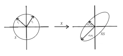
 Singular Value Decomposition of a 2x2 matrix - photo: CenterSpace
The image shows how PCA decomposes data into principal components (directions of maximum variance).
Limitations of PCA
1. Computational Cost
Calculating covariance requires multiplying all samples together, which can be computationally intensive for large datasets.
2. Linear Relationships Only
PCA assumes linear correlations. It struggles with polynomial or exponential relationships. You can apply kernel methods (like kernel PCA) to handle non-linearity, but that adds complexity.
3. Sensitive to Scaling
Variables with larger ranges dominate the analysis. Always standardize first.
Better Alternative: Singular Value Decomposition
There is a more general approach for dimensionality reduction which is also more computationally efficient called Singular Value Decomposition (SVD). I’ll cover this in a future tutorial.
Implementation Resources
For a step-by-step Python implementation, see Nikita Kozodoi’s excellent tutorial.
Quick Example:
import numpy as np
from sklearn.decomposition import PCA

# Your data (100 samples, 50 features)
X = np.random.randn(100, 50)

# Reduce to 10 components
pca = PCA(n_components=10)
X_reduced = pca.fit_transform(X)

# Check explained variance
print(f"Variance explained: {pca.explained_variance_ratio_.sum():.2%}")
When to Use PCA
Use PCA when:
- You have many correlated variables
- You need to visualize high-dimensional data
- You want to speed up machine learning
- You need to remove noise
Don’t use PCA when:
- Variables are already independent
- Non-linear relationships dominate
- You need to interpret individual features
- Data is sparse
Conclusion
PCA is a powerful tool for managing high-dimensional data. By identifying principal components (directions of maximum variance), it reduces complexity while preserving most information. Despite limitations with non-linear data, it remains one of the most widely used techniques in data science.
